The goal of this blogpost is to demonstrate how the formulation of the Variational Autoencoder (VAE) translates to empirical observations using the MNIST dataset. First, we examine how VAEs handle the tasks that their formulation dictates, i.e. reconstruction of their input and generation of samples using the decoder. Then, we study the output distribution of the encoder in the latent space. Last, we use our observations of the latent space and strategically choose the latent variable to generate examples in order to see how the latent space affects the pixel space and the final image.
We assume the reader is familiar with VAEs and the how the formulation is derived and interpreted. If not, we have an in-depth study on the matter.
Let's start by examining the loss function of the VAE:
\[ \begin{equation} \begin{split} \mathcal{L}(\theta, \phi; x) & = D_{KL}(q_{\phi}(z|x) \| p_{\theta}(z)) - \mathbb{E}_{q_{\phi}(z|x)}\left[ \log{p_{\theta}(x|z)} \right] \\ & = D_{KL}(q_{\phi}(z|x) \| p_{\theta}(z)) + \mathcal{L}_{REC}(\theta, \phi; x) \end{split} \end{equation} \]
where \( D_{KL} \) is the KL divergence, \(L_{REC}\) is the reconstruction loss of the input, \(p_{\theta}(z)\) is the prior distribution of the latent code \(z\), usually chosen to be standard normal distribution, \( q_{\phi}(z|x) \) the output distribution of the encoder (which is usually a Gaussian MLP), and \( p_{\theta}(x|z) \) the output distribution of the decoder (which is usually a Bernoulli MLP). The reconstruction loss, therefore, is usually chosen by setting
\[ \log{p_{\theta}(x|z)} = \sum_i x_i\log{\hat{x}_i} + (1 - x_i)\log{(1 - \hat{x}_i)},\]
where \(\hat{x}_i\) is the reconstruction of the VAE of the input \(x_i\). It is easy to see that the formulation of the VAE attempts to minimize the deviation of the output posterior distribution of the encoder from the standard normal distribution while still accurately reconstructing the input.
Architecture
We realize the neural net as a simple feedforward net, where the encoder has one hidden layer of 256 units and outputs a \(n\)-dimensional mean and variance. Likewise, the decoder has a hidden layer of 256 units.
 |
VAE's architecture
|
For the most part, we set \(n=2\) because it allows us to depict the true latent space graphically. Whenever we deviate from that, we explicitly state it. Moreover, we experiment with a conditional VAE (CVAE), a VAE that is where an extra variable is provided as input, both along with the input sample and with the latent code of the decoder. A conditioning variable is usually some important high-level notion that describes the input sample, e.g. its label. In our case, we simply one-hot encode the label and concatenate it with the 784-dimensional input and the \(n\)-dimensional latent code.
Reconstructions
Let's see how well can the VAE reconstruct its input. Below are some input-output pairs.
 |
VAE (\(n=2\)) reconstructions
|
It becomes immediately evident that the reconstructions are blurry. It is also worth mentioning that (in this small sample) the value of the output digit is the same as the input one, i.e. the VAE does not alter the essence of the input. But, more than that, we can see that it manages to retain the general shape of the input too, e.g. in the 3rd reconstruction the output has the same rotation as the input (compared to a "prototypical" vertical 1). It can be argued, however, that constraining the latent space to be a subspace of the 2D plane is too restrictive. Let's see how the VAE fares if we increase \(n\). For \(n=5\), we get:
 |
| VAE (\(n=5\)) reconstructions |
and for \(n = 10\):
 |
| VAE (\(n=10\)) reconstructions |
We do observe an increase in the quality of the reconstruction, the images are sharper now for example. However, the other, stylistic modes of deviation each digit displays are sufficiently captured by the \(n=2\) VAE, which also validates the graphical illustrations that follow for the rest of this study. Note that the inputs were randomly selected from the test set of the VAE.
Generated Samples
However, one of the premises of the VAE is that its decoder can be used solo as a generator, with the latent code sampled from the selected prior distribution. Using the same VAEs as before for \(n=2,5 \) and 10, we get, respectively:
 |
VAE (\(n=2\)) random samples
|
 |
| VAE (\(n=5\)) random samples |
 |
| VAE (\(n=10\)) random samples |
The drop in sample quality is apparent. Not only are the results rough for all the VAEs no matter their latent space dimension, the resulting digits are also ambiguous. Let's explore why that is by peaking at the latent space of the VAE directly.
Latent Space
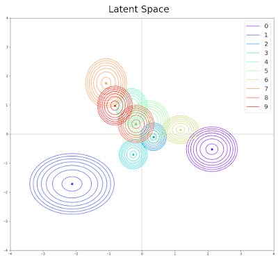
Given an input digit, the encoder produces the mean and the variance of a Gaussian distribution. By averaging several of these estimations per digit (i.e. class), we can estimate with some certainty the distributions of the 10 digits in the latent space, which the decoder in turn has learned to transform into images. We visualize the distributions by drawing several contours of equal probability. For a 2D Gaussian, a contour of equal probability is an ellipse. We draw corresponding contours for each distribution. Therefore, for the VAE, the latent space looks like this:

We can easily see that each digit resides in a different area compared to the rest, even though several of these overlap. It is also clear that each distribution is not close to the prior we set, the standard Gaussian distribution. Intuitively, that would not make sense, as there would not be any means available for the decoder to discern which digit the encoder "saw" and encoded. Thus, the encoder models digits by assigning them a separate space in the latent space, denoted by the mean, and then deviating from it slightly to model the variation within the class. It is for this reason that the generator failed to generate quality examples consistently. Completely random sampling from the prior risks yielding a point equally close to multiple distributions, rendering its reconstruction ambiguous for the generator.
So, to see the actual properties of the generator, let's focus on a single digit. We arbitrarily choose 9. To do so, we empirically find the mean of all 9s as above, and then generate images by moving on a 2D grid centered around that mean. The resulting picture is:
where on the upper left of each digit we note the coordinates used to generate it. We can see that even two steps away from the center the resulting digit begins to become some sort of interpolation between 9 and other digits encoded in the surrounding area. Lets take a close look at how the space is arranged near 9's distribution and verify that the distortions are consistent according to the latent space:
Indeed, on the upper left resides 7, on the right we have 4s and 8s, on the lower left side we have 1s and on the bottom 3s. Let us now see how the picture of the latent space changes when we use two different sets of digits to estimate it:
As expected, it remains consistent. Nonetheless, up to this point, we have been using again the training set of the VAE to visualize the latent space. The test latent space:
also paints the same picture. Fortunately, we have not reached a dead end, not yet.
Conditional VAE
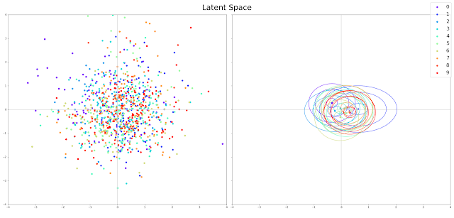
By using the label of the digit as a conditioning variable, we expect to alleviate the burden of encoding the class of the input from the encoder, and the decoding of the class in the latent space from the decoder. But does that expectation adhere to reality? Yes, it does!
The distributions of the digits in the latent space are indistinguishable and truly a standard normal distribution. By biasing the decoder to generate 9s using the corresponding conditioning variable, and then traversing the 2D grid centered at \( (0,0) \):
we can see that the latent space plays no role in determining the value of the output digit, but only affects its style. For instance, as we move from left to right, we can observe that the width of the resulting digit shrinks, while from bottom to top the tail of the digit rotates. Using these observations, we are now able to use the decoder as a generator whose output can be readily controlled via the conditioning variable, while the latent variable can be sampled from the prior with no hesitation. Some example generated samples, which can be presented in a more principled manner now, are:
 |
| CVAE (\(n=2\)) random samples |
And, for \( n = 5 \):
 |
| CVAE (\(n=5\)) random samples |
In general, the quality of the generated samples is better compared to the plain VAE.
Conclusions
In this study, we explored the empirical qualities of the VAE and its formulation. We did so by checking its ability to reconstruct its input, its ability to generate samples given a latent code samples from the prior distribution and the qualities of its latent space. Then, we contrasted that with a CVAE, showing a better generation quality stemming from the extra degree of freedom the conditioning variable grants.


 Download IPython notebook


Comments
Post a Comment